Class 1: Summary Statistics
Key Ideas
A summary statistic reduces a list of numbers to a single number that describes some feature of the list. The four below describe either the center of the data or its spread.
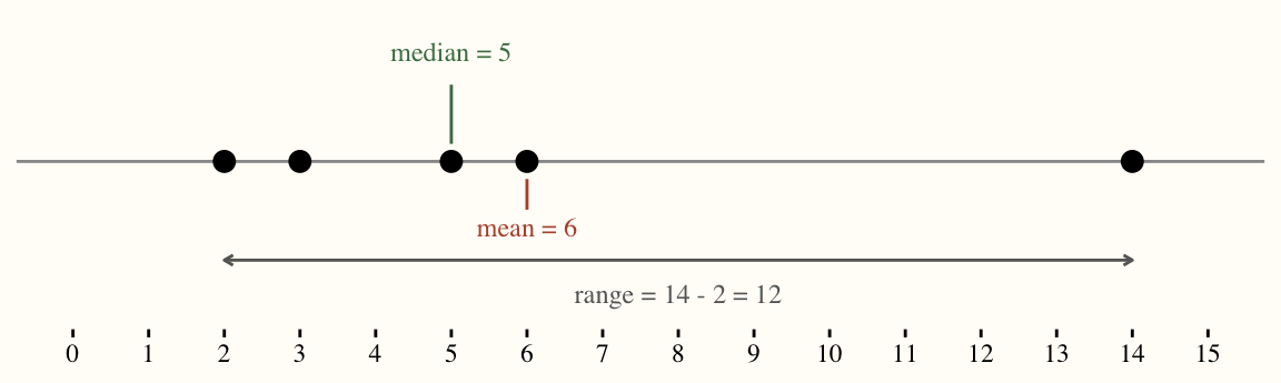
The mean is the arithmetic average: add the values and divide by how many there are, \(\bar{x} = \frac{1}{n}\sum_{i=1}^n x_i\). The median is the middle value once the data are sorted; with an even number of values, it is the average of the two middle values. The mode is the value that occurs most often. Each of these is a measure of central tendency, and they need not agree.
The range is the largest value minus the smallest value. It is a measure of spread rather than of center.
Survey
Please take 10 minutes to complete this class survey. You are welcome to skip any questions you prefer not to answer. Your responses will be anonymous and will not be linked to your name. We will combine everyone’s responses into a single spreadsheet and use that data set for data analysis throughout the course.
QR code to access the survey:

Or URL: https://tinyurl.com/econ005
Problems of the Day
Q1: Half Truths
Are the following statistical statements sometimes, always or never true? Explain, giving examples and/or counterexamples.
- Half of the students taking a test score less than the average mark.
- Nobody scores higher than the average mark in a test.
- Suppose that in a game you can only score an even number of points: 0, 2, 10, 50. So, the average score over a series of games is an even number.
Q2: Mean but Not Meaningful
Here are five responses from the class survey. Using a calculator, compute the average of each column and then interpret it.
| Student | Interest in Data Analysis (1 = low, 5 = high) | Commute (one way, miles) | Work (hours per week) | Birth month | Any pets? |
|---|---|---|---|---|---|
| Ana | 4 | 2 | 0 | 3 (March) | yes |
| Ben | 3 | 15 | 20 | 11 (November) | no |
| Cal | 5 | 0.5 | 10 | 7 (July) | yes |
| Dee | 2 | 40 | 25 | 1 (January) | no |
| Eli | 3 | 5 | 0 | 12 (December) | yes |
If you reported each of these averages to someone who hadn’t seen the data, which of the averages would mislead them, and what would be a better summary in those cases?
Answers
Q1: Half Truths
Sometimes. Half the class scores below the mean only when the mean happens to sit at the median. Scores of 50, 60, 70, 80 have mean 65, and exactly two of four are below it. But scores of 0, 90, 90, 90 have mean 67.5, and three of four are above it: one very low score drags the mean down without moving the median. The statement is usually false whenever the distribution is lopsided, and it is false in the other direction when scores tie: if everyone gets 70, the mean is 70 and nobody is below it.
Sometimes, and only in one situation: when every score is identical. The mean is the balance point of the scores, so if anyone is below it, someone else must be above it to balance them out. The moment two students score differently, at least one is above the mean.
Sometimes. The average of two games scoring 2 and 2 is 2, which is even. But the average of 0 and 2 is 1, which is odd, and the average of 2, 10, and 50 is \(62/3 \approx 20.67\), which is not an integer at all. The mean of a list does not have to be a value that could appear in the list; it does not even have to be a whole number.
Q2: Mean but Not Meaningful
The arithmetic is the same in every column (add, divide by 5), but the interpretation is not.
| Interest | Commute | Work | Birth month | Pets (yes = 1) | |
|---|---|---|---|---|---|
| Sum | 17 | 62.5 | 55 | 34 | 3 |
| Mean | 3.4 | 12.5 | 11 | 6.8 | 0.6 |
- Work hours (mean 11) is a quantity, so the arithmetic is legitimate, but the mean still misleads. Look at the data: 0, 0, 10, 20, 25. Two students do not work at all, and the three who do work between 10 and 25 hours. Nobody works anything like 11 hours. The data are bimodal, with one cluster at zero and another well above it, and a single number in the gap between the clusters describes no one. A better summary keeps the two groups apart: “2 of 5 students do not work; among those who do, the average is about 18 hours.”
- Commute (mean 12.5 miles) is also a quantity, but look at the data: four of the five students commute 5 miles or less, and Dee’s 40-mile drive alone accounts for most of the total. The mean is above what four of five students experience. The median, 5 miles, describes the typical student better, and reporting both (“median 5, mean 12.5”) signals that someone has a long commute.
- Interest in Data Analysis (mean 3.4) is ordered, but the gaps are not guaranteed to be equal: the jump from “2” to “3” need not mean the same thing as from “4” to “5”. An average of 3.4 is a rough summary; reporting the whole distribution (one 2, two 3s, one 4, one 5) is more honest.
- Birth month (mean 6.8) is a label, not a quantity. The mean does not say the typical student was born in late July; nobody except Cal was born anywhere near July. Dee (January) and Eli (December) have birthdays a month apart on the calendar but sit at opposite ends of the scale, and they average to 6.5, which is nonsense. A table of counts, or the mode, is the right summary.
- Pets is a yes/no variable. Coding yes as 1 and no as 0, the mean is 0.6, which is the proportion of students with pets. That is a useful number, but only because of the 0/1 coding. “The average student has 0.6 of a pet” misleads; “60% of students have a pet” does not.
The lesson: before computing an average, ask whether the numbers are measuring an amount of something. If they are codes for categories, the mean is arithmetic without meaning.