Class 5: Covariance and Correlation
Key Ideas
Class 4 described one random variable at a time. Today we describe how two vary together.
Two random variables \(X\) and \(Y\) are independent when learning the value of one leaves the distribution of the other unchanged. Their covariance, \[\text{Cov}(X, Y) = E\big[(X - E[X])(Y - E[Y])\big],\] is the probability-weighted average of the product of the two deviations: positive when \(X\) above its mean tends to come with \(Y\) above its mean, negative when above tends to come with below. In data, the sample covariance is \(s_{xy} = \frac{1}{n-1} \sum (x_i - \bar{x})(y_i - \bar{y})\), by analogy with the sample variance of Q3; R computes it with cov(). The correlation divides the covariance by the product of the two standard deviations, \(r = s_{xy} / (s_x s_y)\), and always lies between \(-1\) and \(1\); R computes it with cor().
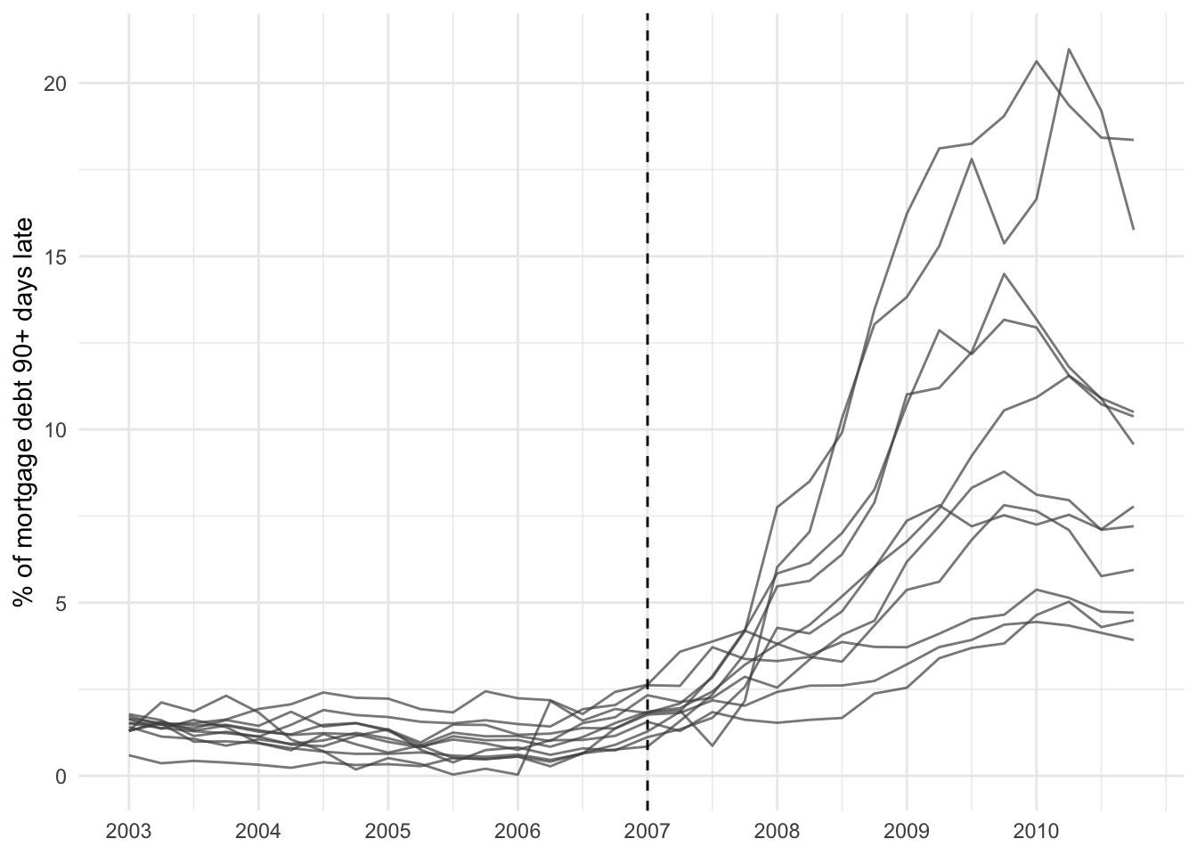
A correlation is one number, estimated from one set of conditions. In the years before 2008, banks bundled thousands of mortgages into securities whose safety rested on one question: if one borrower defaults, how likely is it that others default too? The standard pricing model summarized that dependence with a single correlation estimated from recent data. During a decade of rising house prices, defaults were rare and scattered, the estimated correlations were low, and pools of such mortgages were rated as nearly riskless. When prices fell across the whole country in 2007, borrowers who had never met defaulted for the same reason at the same time. The common cause had been there all along; it had simply been quiet in the data used to estimate the correlation.
Problems of the Day
Q12: Ninety-Six Times Stronger
Three student teams each surveyed four classmates about commute and sleep. Team A recorded miles and hours, Team B kilometres and minutes, Team C miles and hours.
| Team A (mi, h) | Team B (km, min) | Team C (mi, h) | |
|---|---|---|---|
| commute | 2, 4, 6, 8 | 3.2, 6.4, 9.6, 12.8 | 1, 4, 8, 11 |
| sleep | 8, 7, 7, 6 | 480, 420, 420, 360 | 9, 7, 5, 5 |
Dana, the campus paper’s data editor, ran cov(commute, sleep) on each team’s data and got \(-2\) for A, \(-192\) for B, and \(-8\) for C. Her headline: “Team B finds a link 96 times stronger than Team A’s; Team C is in between.” Her editor Marcus refuses to run it: “All three teams found the same thing.” Which team found the strongest relationship, and how strong is it?
Q13: The Same Every Month
Rosa manages campus facilities. For two buildings she has five months of average temperature (°F) and energy bill ($):
| temperature | 30 | 45 | 60 | 75 | 90 |
|---|---|---|---|---|---|
| gym | 290 | 240 | 200 | 110 | 60 |
| library | 300 | 165 | 120 | 165 | 300 |
Given cov(temp, gym bill) = -2212.5, var(temp) = 562.5, and var(gym bill) = 8850, find cor(temp, gym bill).
Why is the covariance of temperature with the library energy bill equal to 0? What does that imply that the correlation between those two variables is?
NoteAnswers
Q12. Team A. Means 5 miles and 7 hours; deviations \((-3, -1, 1, 3)\) and \((1, 0, 0, -1)\); products sum to \(-6\), so \(s_{xy} = -6/3 = -2\). \(s_x = \sqrt{20/3} = 2.58\), \(s_y = \sqrt{2/3} = 0.82\), \(r = -2 / (2.58 \times 0.82) = -0.95\). Team B. The same four students: every commute is \(1.6\times\) Team A’s and every sleep \(60\times\), so the covariance is \(1.6 \times 60 = 96\) times larger (\(-192\)), and so is the product of the standard deviations (\(4.13 \times 49.0 = 202.4\)). \(r = -192/202.4 = -0.95\), identical to Team A. Team C. Means 6 and 6.5; deviations \((-5, -2, 2, 5)\) and \((2.5, 0.5, -1.5, -1.5)\); products \(-12.5, -1, -3, -7.5\) sum to \(-24\), so \(s_{xy} = -8\). \(s_x = \sqrt{58/3} = 4.40\), \(s_y = \sqrt{11/3} = 1.91\), \(r = -8/8.42 = -0.950\). Verdict. Marcus is right about A and B, which are the same data in different units. Dana is right that C is stronger than A, but only by a hair: \(-0.950\) against \(-0.949\), not 24 times. Team C found the strongest relationship, \(r = -0.95\), and so did everyone else. It comes out this way because a covariance carries the units of both variables (mile-hours for Team A, kilometre-minutes for Team B), so changing units changes the number; dividing by the two standard deviations cancels the units and leaves a number only the shape of the cloud can move.
Q13. Gym. \(s_x = \sqrt{562.5} = 23.7\) and \(s_y = \sqrt{8850} = 94.1\), so \(r = -2212.5 / (23.7 \times 94.1) = -2212.5 / 2231 = -0.99\): a nearly perfect straight line sloping down. Library. Mean temperature 60, mean bill $210; deviations \((-30, -15, 0, 15, 30)\) and \((90, -45, -90, -45, 90)\); products \(-2700, 675, 0, -675, 2700\) sum to exactly \(0\), so the covariance is \(0\). The correlation is the covariance divided by two positive standard deviations, so it is \(0\) as well. It comes out this way because the covariance only asks whether above-average temperatures go with above-average bills; in the library the two hot months say yes and the two cold months say no, by exactly the same amount, so they cancel, even though temperature determines the bill completely.