Class 3: Group Means
Key Ideas
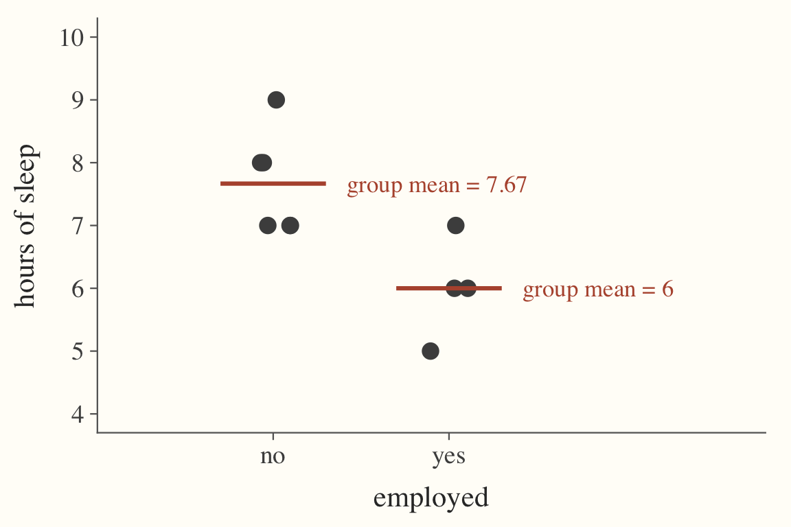
In Class 1 we reduced a whole variable to one number, its mean. Today we compute means within groups, where a group is the set of observations that share one value of a variable. Here is a slice of the class survey: ten students, whether they are employed outside of school, and their nightly hours of sleep.
| student | employed | sleep |
|---|---|---|
| A | no | 8 |
| B | no | 7 |
| C | no | 9 |
| D | no | 7 |
| E | no | 8 |
| F | no | 7 |
| G | yes | 6 |
| H | yes | 7 |
| I | yes | 6 |
| J | yes | 5 |
The group mean of sleep for employed students is the ordinary mean computed using only the rows where employed is yes: \((6 + 7 + 6 + 5)/4 = 6\) hours. For students without jobs it is \(46/6 \approx 7.67\) hours. Each group mean is a mean in the Class 1 sense; what changes is which observations are allowed in.
The difference in means between two groups is one group mean minus the other; here, \(6 - 7.67 = -1.67\) hours. It describes the two groups as they are.
Problems of the Day
Q6: The Guessing Game
A new student joins today. Guess their hours of sleep last night and explain your guess.
I’ll tell you one fact: they have a job. How does your guess change?
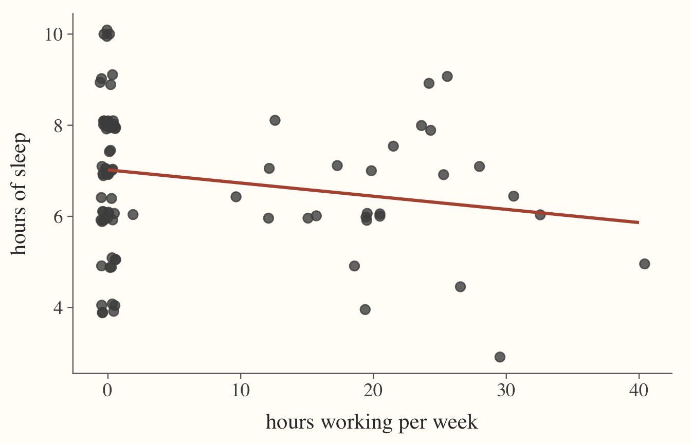
What if I had instead told you that they work more than 30 hours a week? Does your guess change again?
Which single fact about a student (out of the survey questions) would you most want to be told before guessing, and why that one? Which single fact would you least want to be told, and why?
 [1] "year"                   "major"                  "courses"
 [4] "interest_data_analysis" "future_data_use"        "math_confidence"
 [7] "commute_miles"          "employed"               "hours_working"
[10] "extracurriculars"       "exercise_hours"         "sleep_hours"
[13] "wake_time"              "alarms"                 "caffeine"
[16] "cups_caffeine"          "pets"                   "handedness"
[19] "first_gen"              "birth_month"            "gender"
[22] "pet_type"
Q7: Quit Your Job
Employed students in our survey sleep less than students without jobs. A wellness blogger sees the two means and posts: “Want an extra half hour of sleep? Quit your job.”
Compute the difference in mean sleep between the two groups. The blogger is reading it as the sleep a student would gain by quitting. In what way might this be false? What does the difference in means actually show?
# A tibble: 2 × 3
  employed sleep_mean     n
  <chr>         <dbl> <int>
1 No             7.03    67
2 Yes            6.39    28
Q8: The Lost Spreadsheet
The dean’s assistant deleted the raw survey. All that survived is a table she had made earlier: for employed students and for students without jobs, the number of students, their mean hours of sleep, and the proportion with pets.
# A tibble: 2 × 4
  employed sleep_mean pets_proportion     n
  <chr>         <dbl>           <dbl> <int>
1 No             7.03           0.463    67
2 Yes            6.39           0.821    28
The dean needs to know what the class-wide average sleep and proportion with pets is. Can you recover these?
Extension. A classmate averages the two group means and gets a slightly different answer. Under what condition would their shortcut be exactly right?
Answers
Q6: The Guessing Game
No information. With nothing to go on, the best guess is a measure of the centre of the whole class. The mean of the 94 reported sleep values is 6.84 hours, the median is 7 and the mode is 8, so a guess of about 7 hours is defensible. The reasoning is the same as in Class 1: a single number that stands in for a whole variable should sit where the data are thickest.
They have a job. Now the new student belongs to a group, and the relevant number is the group mean rather than the class mean. The 28 employed students average 6.39 hours, so the guess drops to about 6.5. The 66 students without jobs average 7.03, which is why the class mean of 6.84 sits between the two groups, closer to the larger one.
They work more than 30 hours. The natural move is to narrow the group again, but look at who is left: only 2 students in the survey work more than 30 hours, and they average 5.5 hours of sleep. A mean of two observations is barely a mean at all; one student answering differently would move it by half an hour or more. The bins in between do not even line up in order (students working 11 to 20 hours average 6.14, those working 21 to 30 average 6.95), which is a sign that these small groups are mostly noise. A sensible guess moves below 6.39, but not all the way to 5.5. Narrowing the group makes the guess more specific and less reliable at the same time, and the trade-off is governed by the group size.
Which fact to ask for. A useful fact is one that splits the class into groups whose means are far apart, with enough students in each group to trust those means, and with some plausible reason to be related to sleep. In this survey the number of alarms a student sets and the number of courses they take are the strongest candidates (students with 0 or 1 alarm average over 7.25 hours; students with 4 alarms average 6.15), and whether the student has a pet splits the class 7.24 against 6.53, a wider gap than employment. Handedness is the worst choice: the two groups differ by less than a fifth of an hour and there are only 9 left-handed students, so the fact carries no information and the smaller group mean is unreliable anyway. Birth month is nearly as bad. Its twelve groups produce means ranging from 5.71 (May) to 8.06 (October), but with 4 to 11 students per month those differences are what chance alone would produce, and there is no reason to expect a birth month to affect sleep.
Q7: Quit Your Job
The table gives the two group means directly: the 28 employed students average 6.39 hours of sleep and the 67 students without jobs average 7.03, so the difference in means is \(6.39 - 7.03 = -0.64\) hours, about 38 minutes. The blogger’s “half hour” is roughly right as a description of the two groups.
The blogger’s error is the word gain. The difference in means compares two different sets of people, and the students who hold jobs were not picked at random from the class. They differ from the others in ways besides employment: in this survey employed students commute an average of 13.5 miles against 8.3 for everyone else, they set more alarms (2.6 against 2.1), and they are concentrated in the second and fourth years rather than the first. Some of them may have jobs because of circumstances that also cost sleep, such as living far from campus or supporting themselves. If a student quits, the job disappears but the commute and the circumstances do not, so there is no reason to expect them to sleep like a student who never needed the job in the first place. The direction of cause could even run the other way, with students who manage on less sleep being the ones who take on work.
What the difference in means actually shows is exactly what its name says: the employed group, as it is, sleeps 0.64 hours less on average than the unemployed group, as it is. It is a description of two existing groups, not a prediction of what would happen to one person who moves from one group to the other. Turning a difference in means into an effect requires an argument that the two groups were alike in every other way, and here they plainly were not.
Q8: The Lost Spreadsheet
Yes, both can be recovered, because a mean is a total divided by a count and the table contains enough to rebuild the totals. The 67 students without jobs slept a total of about \(67 \times 7.03 \approx 471\) hours and the 28 employed students slept \(28 \times 6.39 \approx 179\) hours, so the class total is about 650 hours over 95 students and the class mean is 6.84 hours. In other words, the class mean is a weighted average of the group means, with each group weighted by its share of the class:
\[\bar{x} = \frac{67}{95}(7.03) + \frac{28}{95}(6.39) \approx 6.84.\]
The larger group pulls the overall mean toward itself, which is why 6.84 sits much closer to 7.03 than to 6.39.
A proportion is a mean of a 0/1 variable (Class 1), so the same trick works, and here the totals are counts of people. A proportion of 0.463 among 67 students means \(67 \times 0.463 \approx 31\) pet owners, and 0.821 among 28 students means \(28 \times 0.821 \approx 23\). That is \(54\) pet owners out of 95, so the class-wide proportion is \(54/95 \approx\) 0.568, or about 57%. Checked against the raw survey, both recovered numbers are right. (One fine point: the sleep mean for the unemployed group was computed with na.rm = TRUE over the 66 students who answered the sleep question, while n() counts all 67 rows. Weighting by 67 gives 6.842 and weighting by 66 gives 6.840, so the slip is harmless here, but it is a reminder that the weights have to be the counts the means were actually computed from.)
Extension. The classmate’s shortcut, \((7.03 + 6.39)/2 = 6.71\) hours and \((0.463 + 0.821)/2 = 0.642\), gives every group the same weight regardless of size. It is exactly right only when the groups are the same size, so that the weights really are one half each. Here the groups are far from equal (67 against 28), so the shortcut misses by 0.13 hours on sleep and by 0.07 on the pet proportion. The error grows with the imbalance in group sizes and with the gap between the group means; if the two groups had the same mean, even badly wrong weights would do no harm.