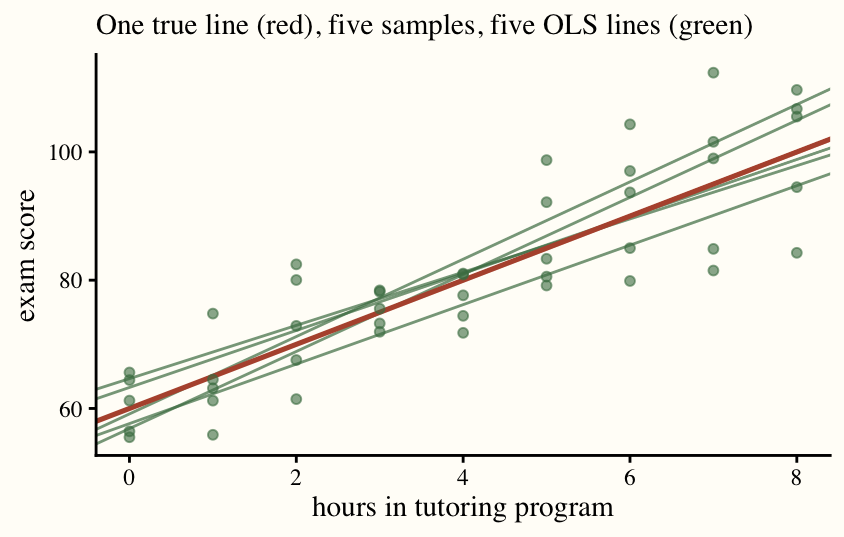
Class 10: Exogeneity
Key Ideas
Class 9 ended with the slope written as a weighted sum of the observed \(y\)’s. Today asks a different kind of question. The number \(\hat{\beta}_1\) is computed from one sample. The number \(\beta_1\) in the data generating process \(y_i = \beta_0 + \beta_1 x_i + u_i\) is a fixed feature of the truth, and nobody observes it. The two are different objects, and the gap between them is the subject of this class.
Because the unobservables \(u_i\) are random, a second sample drawn from the same truth would contain different \(u_i\), different \(y_i\), and therefore a different \(\hat{\beta}_1\). The estimator is a random variable: it has a distribution, an expectation, and a variance, even though we only ever see one draw of it.
The natural question is where these draws land relative to \(\beta_1\). The figure below repeats the sampling many times and records \(\hat{\beta}_1\) from each sample.
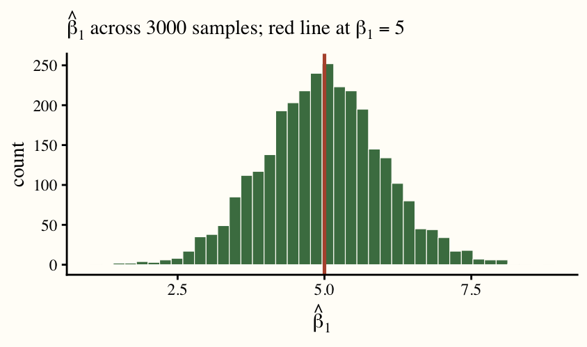
Today’s problems show why the distribution centers where it does, and identify the assumption about \(u\) and \(x\) on which that result depends.
Problems of the Day
Q26: The Gap
Last class you showed \(\hat{\beta}_1 = \dfrac{\sum_{i=1}^n (x_i - \bar{x})\, y_i}{\sum_{i=1}^n (x_i - \bar{x})^2}\). That formula is built from data. The truth, which the data came from, is \(y_i = \beta_0 + \beta_1 x_i + u_i\). This question connects the two. More algebra, but this one pays off: the equation you end with is the one the rest of the quarter is built on.
Step 1: Substitute the truth for \(y_i\) in the numerator and distribute \((x_i - \bar{x})\). You should get three sums: one multiplied by \(\beta_0\), one by \(\beta_1\), and one containing \(u_i\).
Step 2: Show that the \(\beta_0\) sum is zero.
Step 3: Show that \(\sum (x_i - \bar{x})\, x_i = \sum (x_i - \bar{x})^2\). The \(\beta_1\) term now cancels against the denominator.
Step 4: Put the pieces together. With \(w_i\) the leverage from Class 9, you should have
\[\hat{\beta}_1 = \beta_1 + \sum_{i=1}^n w_i u_i.\]
Which side of this equation could you compute from the data, and which only if you knew the true data generating process?
Q27: The Growth Chart
The conditional expectation \(E[X | Y]\) of a random variable is its expected value given that some other variable takes a particular value. For example: a doctor’s height chart for adults in a certain population reads
\[\mathbb{E}[\text{height} \mid \text{sex}] = \begin{cases} 64'' & \text{if female} \\ 69'' & \text{if male.} \end{cases}\]
Compute \(\mathbb{E}[\text{height}]\) if the population is half male.
What if the population is only 1/4 male?
Write a general formula for \(\mathbb{E}[\text{height}]\) in terms of the two conditional expectations \(E[\text{height} | \text{sex = male}]\) and \(E[\text{height} | \text{sex = female}]\). This should remind you of group means from class 3.
Extension. Decide whether the statement below is always, sometimes, or never true.
If \(\mathbb{E}[X \mid Y] = c\) for every value \(Y\) can take, then \(\mathbb{E}[X] = c\).
Q28: Finishing the Proof
From Q26, \(\hat{\beta}_1 = \beta_1 + \sum_{i=1}^n w_i u_i\). An estimator is unbiased if its expectation equals the truth. We now work out when OLS is unbiased.
Step 1: Take the expectation of both sides. Note that the expectation of a sum is the sum of the expectations. What condition needs to hold for \(\hat{\beta}_1\) to be unbiased?
Step 2: \(w_i\) and \(u_i\) are both random, so \(\mathbb{E}[w_i u_i]\) does not split into a product. Instead, condition on \(X\), meaning all the \(x\)’s in the sample. Once \(X\) is fixed, \(w_i\) is a constant and comes out front: \(\mathbb{E}[w_i u_i \mid X] = w_i\, \mathbb{E}[u_i \mid X]\).
Step 3: The exogeneity assumption is \(\mathbb{E}[u_i \mid X] = 0\). Apply it, and then finish the proof that \(\mathbb{E}[\hat{\beta}_1] = \beta_1\).
Write the whole argument as one chain of equalities, each labeled with the fact that justifies it.
Extension. Sharpen Tutoring regresses exam score on hours in its program and advertises the slope as the gain from each hour. Let the truth be \(\text{score} = 60 + 5 \cdot \text{hours} + u\). Sketch the true line and, at each value of hours, a small cloud of students that satisfies exogeneity: \(\mathbb{E}[u \mid \text{hours}] = 0\).
On a second sketch, draw clouds that violate exogeneity and the line OLS would fit through them. What kinds of variables might make \(\mathbb{E}[u \mid \text{hours}]\) rise with hours? Which way would the OLS slope be biased in that case?
The key idea is that when people are able to choose their \(X\) values, exogeneity is rarely satisfied. This is why scientists do randomized controlled trials (RCTs): the scientist randomly assigns people their \(X\) values, and then they observe the outcome. In this way, \(X\) becomes independent of \(U\) and we have exogeneity. Explain what the RCT would be in the tutoring example, and why an RCT would yield a more accurate estimate of the effect compared to observational study.
Observational studies aren’t by definition invalid however: we’ll return to this topic at the end of the course (classes 17-19).
NoteAnswers
Q26: The Gap
Step 1. Replace \(y_i\) by \(\beta_0 + \beta_1 x_i + u_i\) in the numerator and distribute:
\[\sum (x_i - \bar{x})\, y_i = \beta_0 \sum (x_i - \bar{x}) + \beta_1 \sum (x_i - \bar{x})\, x_i + \sum (x_i - \bar{x})\, u_i .\]
Step 2. Deviations from the mean sum to zero: \(\sum (x_i - \bar{x}) = \sum x_i - n\bar{x} = n\bar{x} - n\bar{x} = 0\). The \(\beta_0\) term vanishes.
Step 3. Subtract the two sums: \(\sum (x_i - \bar{x})\, x_i - \sum (x_i - \bar{x})^2 = \sum (x_i - \bar{x})\,[x_i - (x_i - \bar{x})] = \bar{x} \sum (x_i - \bar{x}) = 0\). So the two sums are equal, and the \(\beta_1\) term becomes \(\beta_1 \sum (x_i - \bar{x})^2\), which cancels against the denominator.
Step 4. Dividing what is left by \(\sum (x_j - \bar{x})^2\),
\[\hat{\beta}_1 = \beta_1 + \sum_{i=1}^n \frac{x_i - \bar{x}}{\sum_j (x_j - \bar{x})^2}\, u_i = \beta_1 + \sum_{i=1}^n w_i u_i .\]
The left side is computable from the sample: it is the OLS slope. The right side is not. It contains \(\beta_1\), which nobody observes, and the \(u_i\), which are the unobservables themselves. Only the weights \(w_i\) are known. The equation says the estimate equals the truth plus a weighted sum of the unobservables, and that second term is why the estimate moves from sample to sample.
Q27: The Growth Chart
Half male. \(\mathbb{E}[\text{height}] = \tfrac12 (69) + \tfrac12 (64) = 66.5''\).
One quarter male. \(\mathbb{E}[\text{height}] = \tfrac14 (69) + \tfrac34 (64) = 17.25 + 48 = 65.25''\).
General formula. With \(p\) the share of the population that is male,
\[\mathbb{E}[\text{height}] = p\, \mathbb{E}[\text{height} \mid \text{male}] + (1 - p)\, \mathbb{E}[\text{height} \mid \text{female}] .\]
This is the Class 3 result that the overall mean is the weighted average of the group means, with weights equal to the group shares. The population mean is pulled toward whichever group is larger.
Extension. Always true. Write the overall expectation as the weighted average of the conditional expectations, one weight per value \(y\) that \(Y\) can take:
\[\mathbb{E}[X] = \sum_y \Pr(Y = y)\, \mathbb{E}[X \mid Y = y] = \sum_y \Pr(Y = y)\, c = c \sum_y \Pr(Y = y) = c .\]
A weighted average of numbers that are all equal to \(c\) is \(c\), whatever the weights. (The converse fails: \(\mathbb{E}[X] = c\) does not force every conditional expectation to be \(c\). The height chart has \(\mathbb{E}[\text{height}] = 66.5''\) while neither group averages 66.5’’.)
Q28: Finishing the Proof
Step 1. \(\mathbb{E}[\hat{\beta}_1] = \beta_1 + \sum_{i=1}^n \mathbb{E}[w_i u_i]\), since \(\beta_1\) is a constant and the expectation of a sum is the sum of the expectations. OLS is unbiased exactly when \(\sum_i \mathbb{E}[w_i u_i] = 0\).
Step 2. Conditional on \(X\), each \(w_i\) is a known number and comes out of the expectation: \(\mathbb{E}[w_i u_i \mid X] = w_i\, \mathbb{E}[u_i \mid X]\).
Step 3. Exogeneity sets \(\mathbb{E}[u_i \mid X] = 0\), so every term is zero. The chain, conditional on \(X\):
\[\begin{aligned} \mathbb{E}[\hat{\beta}_1 \mid X] &= \mathbb{E}\Big[\beta_1 + \textstyle\sum_i w_i u_i \,\Big|\, X\Big] && \text{(Q26)} \\ &= \beta_1 + \textstyle\sum_i \mathbb{E}[w_i u_i \mid X] && \text{(expectation of a sum; } \beta_1 \text{ constant)} \\ &= \beta_1 + \textstyle\sum_i w_i\, \mathbb{E}[u_i \mid X] && (w_i \text{ is fixed once } X \text{ is fixed)} \\ &= \beta_1 + \textstyle\sum_i w_i \cdot 0 && \text{(exogeneity)} \\ &= \beta_1 . \end{aligned}\]
The conditional expectation equals \(\beta_1\) for every possible \(X\), so by the Q27 extension the unconditional expectation does too: \(\mathbb{E}[\hat{\beta}_1] = \beta_1\). The histogram in the Key Ideas centers on 5 because that simulation drew \(u\) independently of hours.
Extension. Exogeneity holds. The clouds sit centered on the true line at every value of hours: above-line and below-line students balance at 0 hours, at 1 hour, and so on. An OLS line through such clouds lands near the true line.
Exogeneity fails. Suppose the students who sign up for many hours are also the most motivated, have parents who pay for other help, or attend better schools. Those traits raise scores and live in \(u\), so \(\mathbb{E}[u \mid \text{hours}]\) rises with hours: the clouds drift above the true line at high hours and below it at low hours. OLS fits a steeper line, and the advertised slope overstates the gain from an hour. The reverse is also possible. If struggling students are the ones who sign up, \(\mathbb{E}[u \mid \text{hours}]\) falls with hours and the slope is biased downward, possibly to zero or below even if tutoring helps.
The RCT. Recruit a pool of students and assign hours by lottery: some get 0, some 2, some 5, and so on, regardless of motivation or background. Hours are then independent of everything in \(u\), so \(\mathbb{E}[u \mid \text{hours}] = \mathbb{E}[u] = 0\) by construction, and the Q28 proof applies: the OLS slope is unbiased for the true effect. In the observational study the groups differ in hours and in motivation, and the slope mixes the two; in the experiment the groups differ only in hours plus noise.