Class 7: Intro to Linear Regression
Key Ideas
You already know how to put two variables on a scatterplot, one on each axis, and to draw a line of best fit through the cloud of points by eye. That line is the subject of the rest of the quarter. Linear regression is the name for using it to describe how two variables are related: how much \(y\) tends to change when \(x\) changes, and how closely the points follow the line.
The two variables play different roles. The one on the horizontal axis, \(x\), is the explanatory variable: it is meant to explain part of the variation in \(y\). The one on the vertical axis, \(y\), is the dependent variable: the model treats it as depending on \(x\). In symbols,
\[y_i = \beta_0 + \beta_1 x_i + u_i, \qquad i = 1, \ldots, n.\]
Here \(u_i\) collects the unobservables: everything other than \(x_i\) that \(y_i\) depends on. We call \(u_i\) “unobservables” because they are things that we either are totally unable to accurately measure, or that we simply didn’t measure. They are not in the data set.
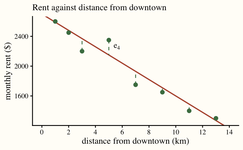
Once a line \(\hat{y} = b_0 + b_1 x\) is drawn, each point sits above or below it; the signed vertical gaps \(e_i = y_i - \hat{y}_i\) are the residuals. Residuals are our estimate of the unobservables. The estimate is only as good as the model: if the model is incorrect or badly estimated, the residuals inherit the line’s mistakes and can be a poor guide to \(u_i\).
Example. Take \(n\) apartments in one city, with \(y_i\) the monthly rent and \(x_i\) the distance from downtown in km. If we draw a scatterplot with distance from downtown on the x-axis and rent on the y-axis and we draw a line of best fit through that scatterplot, we might get something like this:
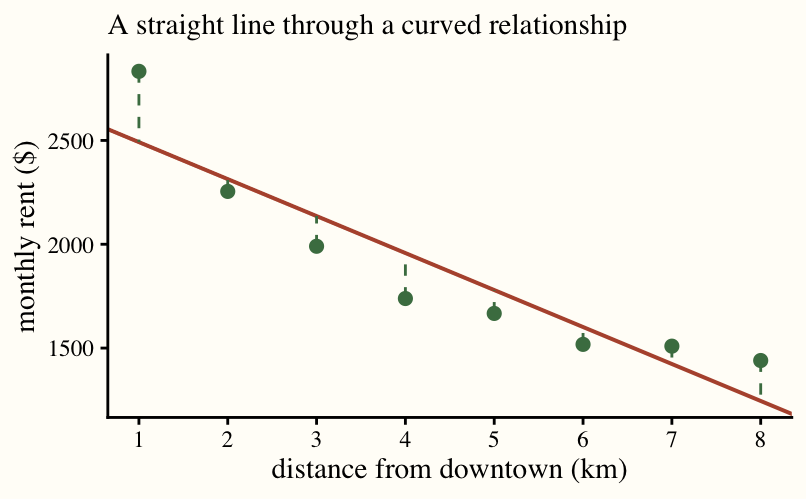
We’d expect the slope (\(\hat{\beta}_0\)) to be negative because, in general, rent falls the further you are from downtown. Unobservables might include floor area, building age, and the view: anything that drives rent (y) that is not included in the right hand side (x). If an observation is above the line of best fit, the residual is positive, perhaps because the apartment is large, new, or has a wonderful view. But perhaps it’s because the model is misspecified:
Problems of the Day
Q17: Two Numbers
Five students report how many hours they studied for an exam and the score they got.
| hours (\(x\)) | 1 | 2 | 4 | 6 | 7 |
|---|---|---|---|---|---|
| score (\(y\)) | 56 | 59 | 72 | 78 | 85 |
Write the code you would use to draw this as a scatterplot in R. Then carefully sketch the scatterplot in your notes. Draw a line of best fit through it by eye and estimate the line’s y-intercept and slope as best you can. Compare with your neighbors: did you get the same values?
Now interpret. Write one sentence each saying what your intercept and your slope mean for students and exams, with units.
A sixth student studied 5 hours; what score does your line predict for them, and what does that number represent if you imagine many students who all studied 5 hours?
Q18: Everything Else
Write the regression model \(y_i = \beta_0 + \beta_1 x_i + u_i\) for the exam data in Q17, saying in words what \(y_i\), \(x_i\), and \(i\) stand for. Then brainstorm at least five things, other than hours studied, that affect a student’s exam score. Where does each of them live in the model?
Now return to the line you drew in Q17. For each of the five students, compute the residual \(e_i\): the vertical distance from the point to your line, with a sign. Which students are above the line and which are below? What do your residuals add up to?
Why is this wrong? “My residual for student 2 is \(-1\), so \(u_2 = -1\): the things that aren’t in the model cost that student 1 point.”
Q19: Summation Statements
Are the following statements always, sometimes, or never true? For “always,” write out both sides with \(n = 3\) and show they are the same expression. For “sometimes” or “never,” give numbers that break it.
Two examples to get you going:
Example #1: \(\sum_{i=1}^{n} (x_i + y_i) = \sum_{i=1}^{n} x_i + \sum_{i=1}^{n} y_i\) is always true. Here’s why:
\[\begin{align} &\sum_{i=1}^{n} (x_i + y_i) = (x_1 + y_1) + (x_2 + y_2) + (x_3 + y_3)\\ &\sum_{i=1}^{n} x_i + \sum_{i=1}^{n} = (x_1 + x_2 + x_3) + (y_1 + y_2 + y_3) \end{align}\]
The only difference between the left and right hand sides is the order of the same six terms.
Example #2: \(\sum_{i=1}^{n} c\, x_i = c \sum_{i=1}^{n} x_i\) for the constant \(c\) is always true.
\[\begin{align} &\sum_{i=1}^{n} c x_i = c x_1 + c x_2 + c x_3\\ & c \sum_{i=1}^{n} x_i = c(x_1 + x_2 + x_3) \end{align}\]
The only difference between the left and right hand sides is that you can distribute \(c\) across terms.
- \(\sum_{i=1}^{n} c = c\)
- \(\sum_{i=1}^{n} x_i y_i = \sum_{i=1}^{n} x_i \sum_{i=1}^{n} y_i\)
- \(\sum_{i=1}^{n} x_i^2 = \left(\sum_{i=1}^{n} x_i\right)^2\)
- \(\sum_{i=1}^{n} (x_i - \bar{x}) = 0\), where \(\bar{x}\) refers to the mean, so \(\bar{x} = \frac{\sum_{i=1}^{n} x_i}{n}\)
- \(\sum_{i=1}^{n} (a + b x_i) = n a + b \sum_{i=1}^{n} x_i\)
NoteAnswers
Q17: Two Numbers
The code.
library(tidyverse)
exams <- tibble(hours = c(1, 2, 4, 6, 7),
                score = c(56, 59, 72, 78, 85))
exams |>
  ggplot(aes(x = hours, y = score)) +
  geom_point()
The line. Any carefully drawn line should land near an intercept of 50 and a slope of 5. Neighbors will not get identical values, and that is the point: “by eye” is a judgment call, so two people looking at the same five points draw two slightly different lines. (The line that minimizes the squared residuals, which we will learn to compute later in the quarter, is \(\hat{y} = 50.8 + 4.81x\).) The rest of these answers use the round version \(\hat{y} = 50 + 5x\).
Interpretation. Intercept: a student who studies 0 hours is predicted to score about 50 points. Slope: each additional hour of studying is associated with about 5 more points on the exam. Units matter here: the intercept is in points, the slope is in points per hour.
Prediction. At 5 hours, \(\hat{y} = 50 + 5 \times 5 = 75\). No individual student is predicted to score exactly 75; some who studied 5 hours will do better and some worse. The 75 is the line’s estimate of the average score among many students who all studied 5 hours. That is the same object as the conditional means from Class 6, except that the line fills in a value for every \(x\), including values like 5 where there is no data at all.
Q18: Everything Else
The model. \(\text{score}_i = \beta_0 + \beta_1 \, \text{hours}_i + u_i\) for \(i = 1, \ldots, 5\). The index \(i\) labels the student, \(y_i\) is student \(i\)’s exam score, and \(x_i\) is the hours student \(i\) studied.
Everything else. Prior knowledge of the material, sleep the night before, attendance, how efficiently the hours were spent, test anxiety, whether the questions happened to hit the topics they knew, tutoring, illness. Every one of them lives in \(u_i\). None is in the data set, so none can appear on the right-hand side; the model sweeps them all into one unobservable term per student.
Residuals from \(\hat{y} = 50 + 5x\):
| student | hours | score | \(\hat{y}\) | \(e_i\) |
|---|---|---|---|---|
| 1 | 1 | 56 | 55 | \(+1\) |
| 2 | 2 | 59 | 60 | \(-1\) |
| 3 | 4 | 72 | 70 | \(+2\) |
| 4 | 6 | 78 | 80 | \(-2\) |
| 5 | 7 | 85 | 85 | 0 |
Students 1 and 3 are above the line; students 2 and 4 are below; student 5 sits on it. The residuals sum to exactly \(0\): the points above the line are balanced by the points below it. Students with different lines will get different sums, and a line drawn well by eye should give a sum near zero. Nothing forces an eyeballed line to balance exactly; the least squares line does, and the residuals from \(\hat{y} = 50.8 + 4.81x\) (\(0.4, -1.4, 2.0, -1.6, 0.6\)) also sum to zero.
Why is this wrong? \(u_2\) is unobservable: it is defined relative to the true \(\beta_0\) and \(\beta_1\), which nobody knows. The residual \(e_2\) is computed from one person’s hand-drawn line, so it mixes two things, the true \(u_2\) and the error in that line. The quickest evidence is in the room: neighbors drew different lines and got different residuals for student 2, and they cannot all be the one true \(u_2\). The residual is an estimate of the unobservable, and it is only as good as the line it came from.
Q19: Summation Statements
- Never true (apart from the special cases \(n = 1\) or \(c = 0\)). With \(n = 3\), \(\sum_{i=1}^{3} c = c + c + c = 3c\). In general \(\sum_{i=1}^{n} c = nc\): a constant added \(n\) times is \(n\) copies of it.
- Sometimes true, rarely. With \(n = 3\) the left side has three terms, \(x_1 y_1 + x_2 y_2 + x_3 y_3\), and the right side has nine, \((x_1 + x_2 + x_3)(y_1 + y_2 + y_3)\). Take \(x = (1, 1)\) and \(y = (1, 1)\): left \(2\), right \(4\). It happens to hold for \(x = (1, -1)\), \(y = (1, 1)\), where both sides are \(0\), but that is a coincidence of the numbers, not a rule. A sum of products is not a product of sums.
- Sometimes true, rarely. \((x_1 + x_2 + x_3)^2 = x_1^2 + x_2^2 + x_3^2 + 2x_1 x_2 + 2x_1 x_3 + 2x_2 x_3\), so the two sides differ by the cross terms. \(x = (1, 1)\): left \(2\), right \(4\). It holds when all but one \(x_i\) is zero, as with \(x = (1, 0, 0)\). Squaring does not distribute over addition.
- Always true. \(\sum_{i=1}^{3} (x_i - \bar{x}) = (x_1 + x_2 + x_3) - 3\bar{x}\), and \(3\bar{x} = x_1 + x_2 + x_3\) by the definition of the mean, so the difference is \(0\). Check with the exam hours: the mean is 4 and the deviations \(-3, -2, 0, 2, 3\) sum to zero. Deviations from the mean always cancel, which is why the mean is the balance point of the data. (The residuals in Q18 are deviations from a line rather than from a mean; the least squares line is the one that makes them cancel too.)
- Always true. Split the sum using Example #1, then apply item 1 to the \(a\)’s and Example #2 to the \(b x_i\)’s: \(\sum_{i=1}^{3} (a + b x_i) = (a + b x_1) + (a + b x_2) + (a + b x_3) = 3a + b(x_1 + x_2 + x_3)\).