Q3: Equally Rested?
For both groups the minimum is 4, the maximum is 10, the range is 6, and the mean is 7, yet the groups are not alike. Group A (4, 7, 7, 7, 10) is mostly clustered at 7, with one short sleeper and one long sleeper, while Group B (4, 4, 7, 10, 10) is split, with nearly everyone at either 4 or 10. The four summaries cannot see this because the range only looks at the two extremes and the mean only looks at the total. The hint points to the deviations from the mean, \(x_i - \bar{x}\): for Group A these are \(-3, 0, 0, 0, 3\) and for Group B they are \(-3, -3, 0, 3, 3\). Group B has more observations far from the mean, which is exactly the feature we want to capture, but both lists sum to zero (the negatives exactly cancel the positives), so averaging the deviations tells us nothing.
The fix is to make the deviations positive before averaging, and squaring is the standard choice. For Group A the squared deviations are \(9, 0, 0, 0, 9\), which sum to 18. For Group B they are \(9, 9, 0, 9, 9\), which sum to 36. Group B’s total is twice as large, matching our intuition that B is more spread out. To turn a total into a typical value we divide by the number of observations, with one twist: statisticians divide by \(n - 1\) rather than \(n\). So we get \(18/4 = 4.5\) for A and \(36/4 = 9\) for B. This quantity is the sample variance, written \(s^2\):
\[s^2 = \frac{1}{n-1}\sum_{i=1}^{n}(x_i - \bar{x})^2.\]
Why \(n - 1\) and not \(n\)? The short version is that the deviations are measured from \(\bar{x}\), which was itself computed from the same five numbers, and that makes them come out a hair too small on average; dividing by a slightly smaller number corrects for it. We will return to this later in the course, and for now you can take it as the convention. Because squaring changes the units (hours become hours squared), we usually take the square root to get back to hours: \(\sqrt{4.5} \approx 2.1\) for A and \(\sqrt{9} = 3\) for B. That square root is the sample standard deviation \(s\). Taking absolute values instead of squaring also works and is a perfectly good invented measure; squaring is simply what statisticians settled on, for reasons we will see later in the course.
Q4: The Dean’s Five Questions
Each question pairs with exactly one tool, and the pairing is decided by how many variables are involved and whether each is categorical or numeric.
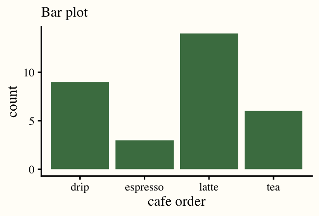
1. Pets: bar plot. Pet type is one categorical variable, so one bar per category. Dogs tower over everything else (28 students), then dog-and-cat households (7), cats alone (6), and a scattering of birds and fish. The point of the picture is the comparison of bar heights, which is why a bar plot works and a histogram does not: there is no numeric axis to bin.
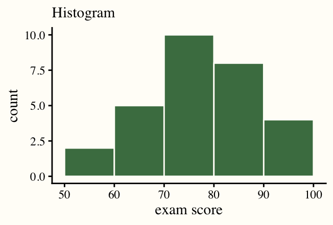
2. Sleep, and is 7 typical: histogram. Sleep is one numeric variable. With one-hour bins the tallest bar is at 8 hours (25 students), followed by 6 hours (20) and 7 hours (15), and the distribution runs from 3 to 10. The median is 7, so in that sense 7 is typical, but the histogram shows something a single number hides: the class splits into a 6-hour crowd and an 8-hour crowd, and only about a quarter of students report between 6.5 and 7.5 hours. “Typical” is a claim about the whole shape, and the histogram is the tool that shows shape.
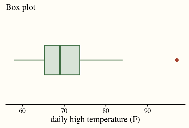
3. Sleep by year: box plot. One numeric variable (sleep) compared across the groups of one categorical variable (year), so one box per year, side by side. From the summary table, first, second and fourth years all have a median near 7 with a box running from about 6 to 8; third years sit lower, with a median around 6 and a box from about 5 to 7. First years have by far the longest whiskers, from 4 up to 10, partly because there are more of them. Five side-by-side boxes make this comparison in one glance, which is what the dean asked for.
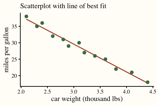
4. Commute and sleep: scatterplot. Two numeric variables, so one point per student at (commute, sleep). In the ten students shown, the points form a loose cloud: a 20-mile commuter sleeps 4 hours, but so does someone with no commute, and the 25-mile commuter gets 7. There is no clear downward drift, so the honest answer is that any relationship is weak in this sample.
5. A 12-mile commuter: scatterplot with a line by eye. A prediction needs a line. Drawn through the cloud in question 4, the line comes out nearly flat at about 6.5 hours, so the dean should expect roughly 6.5 hours of sleep. The scatter around the line runs from 4 to 9 hours, though, so the prediction says more about the class average than about any one student. The line is what turns a picture of a relationship into a number, which is why it is a separate tool from the plain scatterplot.
Q5: The Night Before Challenger
The engineers’ chart. Only seven flights had damage: temperatures 53, 57, 58, 63, 70, 70 and 75, with damage counts 2, 1, 1, 1, 1, 1, 2. Plotted, these seven points are a flat smear. The two flights with the most damage sit at 53°F and 75°F, the coldest and the warmest of the seven, so temperature appears to have nothing to do with it. That is what NASA saw.
The chart they should have drawn. All 23 flights. Now sixteen zero-damage flights appear, and every one of them was launched at 66°F or warmer. Every flight below 66°F had damage (four out of four), while only three of nineteen flights at 66°F or above did. The pattern is stark: damage is a cold-weather problem.
What changed and why it mattered. Nothing about the seven damaged flights changed; the missing information was the comparison group. To show that cold causes damage you have to show that warmth avoids it, and the only evidence of that lives in the boring flights where nothing happened. Selecting on the outcome (keeping only flights with damage) threw away exactly the observations that carried the signal. This is the same lesson as the box plot in Q4: a difference between groups is invisible if you only look at one group.
Extension. A line by eye through the full scatterplot slopes downward, from near zero damaged O-rings at 80°F to a little over one at 53°F, and reading it off at 31°F gives roughly two damaged O-rings. That number deserves very little trust. It is an extrapolation: 31°F is 22 degrees colder than any shuttle had ever flown, and nothing in the data says the pattern stays a straight line that far out. It could be much worse. The line also ignores that there are six O-rings, so damage cannot grow forever, and it rests on just four cold launches. What the engineers should have said is what the honest chart says on its own: every launch below 66°F showed damage, the trend gets worse as it gets colder, we have never flown anywhere near 31°F, and we have no evidence it is safe. The burden was to show safety, not to predict a count.