Class 11 ended with \(\text{Var}(\hat{\beta}_1) = \sigma^2 / \sum (x_i - \bar{x})^2\). The denominator is a sum over the data. The numerator is the variance of the errors \(u_i\), which nobody observes, so the formula cannot be evaluated from a data set. Today replaces \(\sigma^2\) with something computable and then asks whether the replacement can be trusted.
To answer that we need a tool that has been implicit since Class 10: a simulation. Whenever we said “imagine drawing another sample from the same truth,” this is how it is done. We choose the truth ourselves, then let the computer play the role of the unobservables. The function rnorm(n, mean = 0, sd = s) draws \(n\) numbers from a normal distribution with that mean and standard deviation, and every call gives fresh draws:
Each row is one set of six unobservables, hovering around zero with a typical size of about 0.64. Feeding a row into the model equation makes one simulated class:
score =4.17+1.38* hours +rnorm(6, sd =0.64)
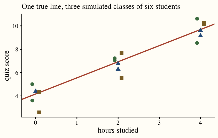
This is \(y_i = \beta_0 + \beta_1 x_i + u_i\) typed out, with \(\beta_0 = 4.17\), \(\beta_1 = 1.38\) and \(u_i \sim N(0, 0.64^2)\). Three runs of it, at the same six values of hours, give the three classes below: one true line, three different clouds.
The point of a simulation is that, unlike with real data, we know \(\beta_1\). So we can run the regression on each cloud and see how close the machinery gets to the truth it was aimed at.
Problems of the Day
Q32: Your Turn at Exogeneity
Let’s practice evaluating the exogeneity assumption, \(\mathbb{E}[u_i \mid X] = 0\). In the regression \(\text{score} \sim \text{hours}\), the variables in \(u\) include motivation, test-taking skill, and previous knowledge. Exogeneity means, in this case, that motivation, test-taking skill, and previous knowledge neither rise nor fall with hours of studying. That is not plausible here: more motivated students study more, and students with better test-taking skill may study less.
Suppose the true \(\beta_1\) is 5: an hour of studying delivers 5 more points on the test. If we estimate \(\hat{\beta}_1 = 15\), that may be because the more motivated students are the ones studying more. It is not the studying that delivers the extra points; the motivated students study more and score higher, and the regression credits hours for both. If instead we estimate \(\hat{\beta}_1 = -5\), that may be because the students with the best test-taking skill study the least: they score well regardless, and the regression reads their low hours and high scores as studying hurting.
The ideal RCT would create treatment and control groups, assign each group a number of hours to study, and compare their average scores. Hours would then have nothing to do with motivation or skill, and the difference in scores would reflect studying alone.
Now your turn. Take the regression \(\text{earnings} \sim \text{schooling}\), annual earnings at age 40 on years of schooling completed, and answer:
What does exogeneity mean in this case?
What do you think the true \(\beta_1\) is?
If we estimated a much higher \(\beta_1\), what violation of exogeneity would explain that?
Explain how the ideal RCT would work to recover the true \(\beta_1\).
Q33: The Missing Ingredient
Last class ended with \(\text{Var}(\hat{\beta}_1) = \sigma^2 / \sum (x_i - \bar{x})^2\). One piece of that formula you could compute from data and one you could not. Which is which, and why?
We never see the errors \(u_i\), but we do see their estimates, the residuals \(e_i\). The estimator of \(\sigma^2\) is
Why \(n - 2\)? Recall Q3, where you invented the sample variance, and Q12, the sample covariance. Both divide by \(n - 1\) rather than \(n\) because the deviations are measured from the sample mean \(\bar{x}\) instead of the true mean of the distribution. The sample mean sits in the middle of this sample, so the deviations from it come out a hair too small; measured from the true mean they would likely be a little bigger, and dividing by \(n - 1\) instead of \(n\) makes up the difference. The same thing happens here, only more so: residuals are measured from a fitted line, and OLS chose both \(\hat{\beta}_0\) and \(\hat{\beta}_1\) to make them as small as possible. Two estimated quantities instead of one, so we subtract 2.
Plugging \(\hat{\sigma}^2\) in for \(\sigma^2\) gives the standard error of the slope, \(se(\hat{\beta}_1) = \sqrt{\hat{\sigma}^2 / \sum (x_i - \bar{x})^2}\). Compute it for the Class 8 data (below), where you estimated \(\hat{\beta_0} = 1.5\) and \(\hat{\beta_1} = \frac{5}{4}\):
\(x\)
\(y\)
\(\hat{y}\)
\(e\)
0
1
2
5
4
6
Check your answer in R:
library(tidyverse)tibble(x =c(0, 2, 4), y =c(1, 5, 6) ) |>lm(y ~ x, data = _) |> broom::tidy()
# A tibble: 2 × 5
  term        estimate std.error statistic p.value
  <chr>          <dbl>     <dbl>     <dbl>   <dbl>
1 (Intercept)     1.5      1.12       1.34   0.408
2 x               1.25     0.433      2.89   0.212
NoteAnswers
Q32: Your Turn at Exogeneity
Exogeneity.\(u\) holds everything else that moves earnings: ability, conscientiousness, conformity, family wealth and connections, health, where a person lives, the industry they work in, luck. Exogeneity says that none of these rise or fall with years of schooling. People with 16 years of schooling would have to be, on average, no abler, no better connected, and no healthier than people with 12.
The true slope. Positive. A year of schooling teaches skills that employers pay for and opens doors to jobs that require credentials. Something like $3,000 to $5,000 of annual earnings per year of schooling is a reasonable guess; estimates in the literature cluster around 8 to 10 percent per year.
A much higher estimate. The people with more schooling would have to be earning more for other reasons. Ability and family background are the natural culprits: abler students stay in school longer and would earn more with or without the degree, and wealthy families both pay for more schooling and supply the connections that land good jobs. Schooling then gets credit for earnings that ability and connections delivered. The omitted variable moves with schooling and with earnings, so the bias is upward.
The ideal RCT. Assign each child a number of years of schooling by lottery, 10, 12, 14, or 16, and enforce it, then record earnings at age 40. Ability, family wealth, and outside opportunities would be spread evenly across the four groups, \(\mathbb{E}[u \mid \text{schooling}]\) would be zero in each, and the difference in average earnings across groups would be the effect of schooling alone. It cannot be run because nobody can be made to leave school at 16, or kept in it, for the sake of an estimate.
The regression on real data compares people who chose different amounts of schooling; the experiment compares people who were handed different amounts, and only the second isolates what schooling does.
Q33: The Missing Ingredient
The two pieces.\(\sum (x_i - \bar{x})^2\) uses only the \(x\)’s, which are in the data set. \(\sigma^2 = \text{Var}(u_i)\) is the variance of the errors, the gaps between each \(y_i\) and the true line. The true line is unknown, so the errors are never seen and \(\sigma^2\) cannot be computed from data.
The table.\(\hat{y} = 1.5 + 1.25x\) gives fitted values \(1.5, 4, 6.5\) and residuals \(e = y - \hat{y}\) of \(-0.5, 1, -0.5\) (they sum to zero, as OLS residuals must).
\(x\)
\(y\)
\(\hat{y}\)
\(e\)
0
1
1.5
\(-0.5\)
2
5
4
\(1\)
4
6
6.5
\(-0.5\)
The standard error.\(SSR = 0.25 + 1 + 0.25 = 1.5\), so \(\hat{\sigma}^2 = 1.5/(3 - 2) = 1.5\). With \(\bar{x} = 2\), \(\sum (x_i - \bar{x})^2 = 4 + 0 + 4 = 8\), and \(se(\hat{\beta}_1) = \sqrt{1.5/8} = \sqrt{0.1875} \approx 0.433\), which is the std.error R prints in the x row. (The intercept’s 1.12 comes from a different formula and is not needed here.)