Class 11: Distribution of Regression coefficients
Key Ideas
Many quantities in nature and in data follow the same bell-shaped curve. The normal distribution \(N(\mu, \sigma^2)\) is fully described by two numbers: its mean \(\mu\), where the peak sits, and its variance \(\sigma^2\), which sets how wide the bell is. An enormous number of variables in nature are approximately normal: adult heights, birth weights, blood pressure, the errors in repeated measurements of the same quantity, the daily temperature on a given date, and countless others. Wherever a histogram of real data is drawn, the bell shape is the usual sight, not the exception.
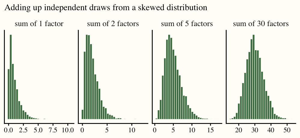
Why does one shape appear so often? The central limit theorem says that when a quantity is the sum of many small, roughly independent influences, its distribution is close to normal, whatever the individual influences look like. Height accumulates many genes and many years of nutrition; an exam score accumulates many topics learned or missed. The figure below starts from a lopsided distribution and adds independent copies of it.
Now recall Q26: \(\hat{\beta}_1 = \beta_1 + \sum_{i=1}^n w_i u_i\). The OLS slope is exactly such a sum, one term per observation. So \(\hat{\beta}_1\) is approximately normal, centered at \(\beta_1\) under exogeneity (Class 10), with a variance still to be found. In the simulation below the errors \(u_i\) are deliberately far from normal, yet the slope is not.
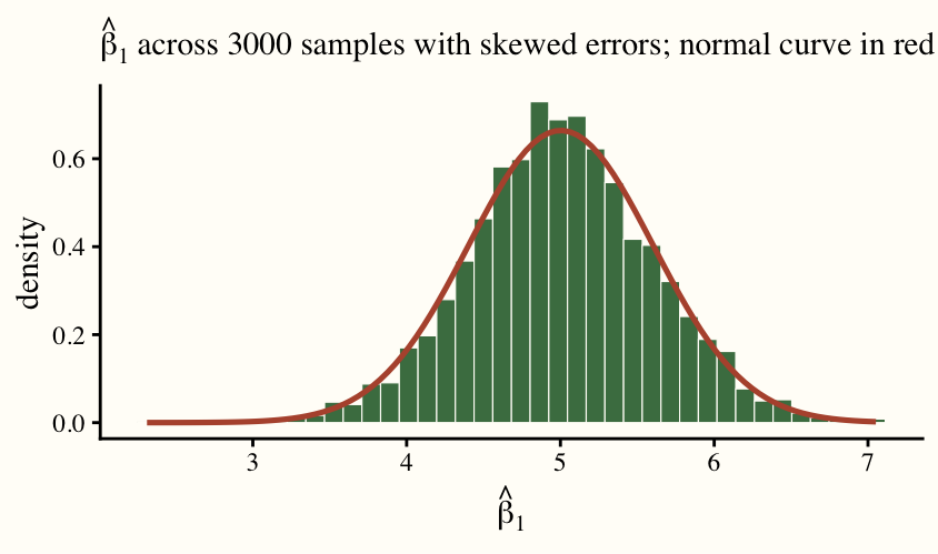
Today’s problems put numbers on the mean and variance of a normal distribution, derive the variance of \(\hat{\beta}_1\), and ask what research design choices make that variance small.
Problems of the Day
Q29: Into the Normal Distribution
This chart accurately shows the probability density functions for three normal distributions:
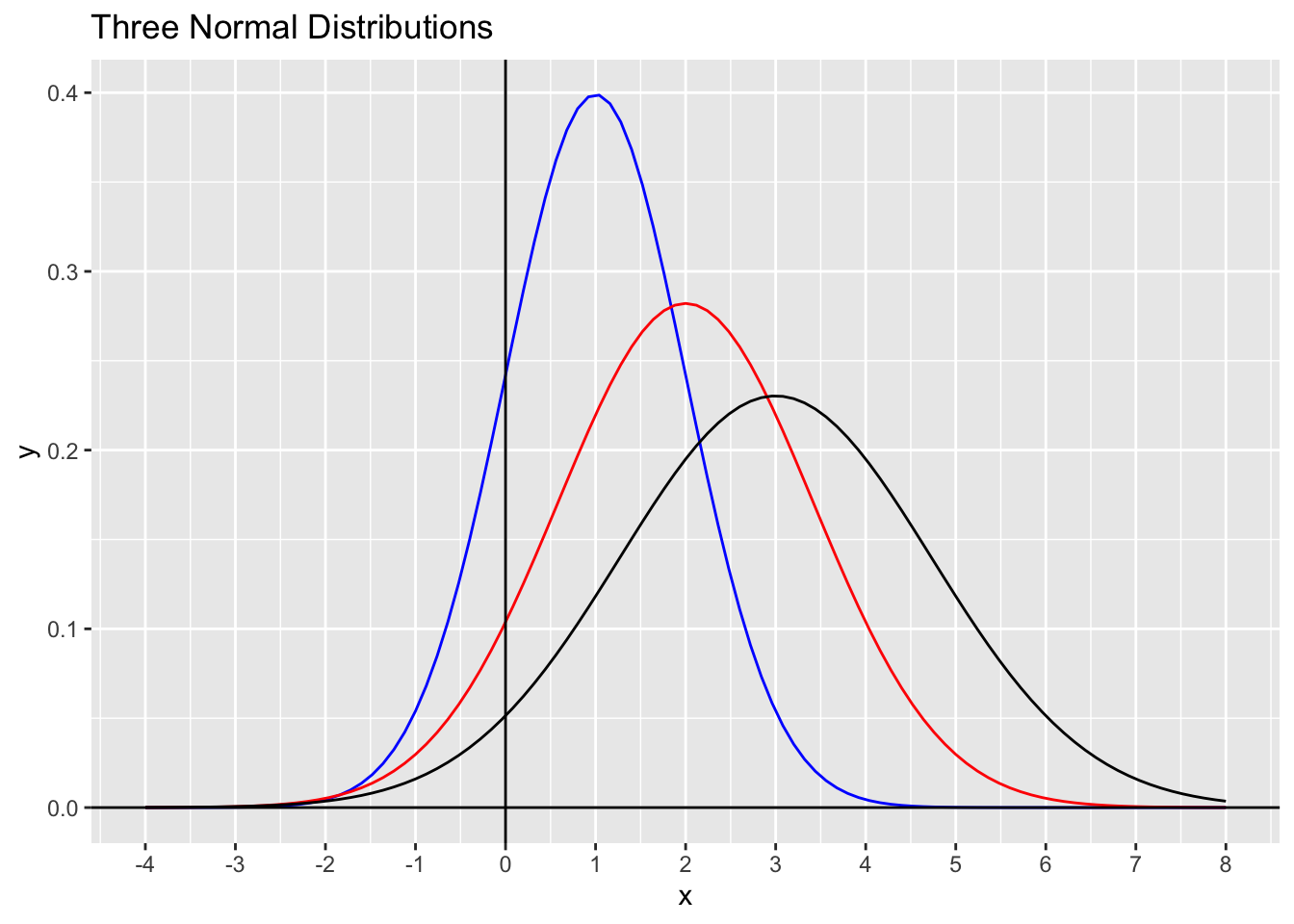
I estimate that the probability that a variable drawn from the blue distribution is negative 25% of the time. Can you suggest how I made this estimate? Is it likely to be an over- or under-estimate?
How about the probabilities that random variables drawn from the other distributions are negative?
My friend says that the means and variances of these normal distributions are whole numbers. Can you calculate those means and variances for each of the normal distributions above? Note that, for a normal distribution, about 95% of the distribution falls within 2 standard deviations of the mean. That leaves only about 5% more than 2 standard deviations away from the mean, with about 2.5% in each tail. Almost all of the distribution falls within 3 standard deviations of the mean, leaving less than 0.3% outside that range.
Q30: The Two Archers
Two archers both hit the bullseye on average. One lands every arrow within an inch of it; the other scatters arrows across the whole target. Class 10 showed OLS is unbiased under exogeneity: it’s centered on the truth. It said nothing about which archer OLS is. For that we need \(\text{Var}(\hat{\beta}_1)\).
Three variance rules, for a constant \(c\) and random variables \(Z\), \(Z_1\), \(Z_2\): \(\text{Var}(c + Z) = \text{Var}(Z)\); \(\text{Var}(cZ) = c^2\,\text{Var}(Z)\); and if \(Z_1\) and \(Z_2\) are independent, \(\text{Var}(Z_1 + Z_2) = \text{Var}(Z_1) + \text{Var}(Z_2)\). Say in one sentence each why these make sense.
Step 1: Start from Q26, \(\hat{\beta}_1 = \beta_1 + \sum_{i=1}^n w_i u_i\), and apply the first rule.
Step 2: In a random sample, why is it reasonable to treat different students’ errors as independent? Apply the third rule to break up the variance of the sum.
Step 3: Condition on \(X\), as in Q28, then apply the second rule to each term. You should have \(\text{Var}(\hat{\beta}_1 \mid X) = \sum_{i=1}^n w_i^2\, \text{Var}(u_i \mid X)\).
Step 4: Assume homoskedasticity: \(\text{Var}(u_i \mid X) = \sigma^2\), the same constant at every value of \(x\). Pull \(\sigma^2\) out front and simplify \(\sum w_i^2\) (square the leverage; the denominator does not depend on \(i\)). You should get
\[\text{Var}(\hat{\beta}_1) = \frac{\sigma^2}{\sum_{i=1}^n (x_i - \bar{x})^2}.\]
Extension. Suppose we somehow knew \(\sigma^2 = 2\), and \(x = \{0, 2, 4\}\). Compute \(\text{Var}(\hat{\beta}_1)\) and its square root, the standard deviation. If you estimated \(\hat{\beta}_1 = 1.25\), how far should anyone trust it (assuming \(\hat{\beta}_1\) is distributed according to the normal distribution)? What kind of archer is OLS in this case?
Q31: Three Levers
Nadia has funding to survey 30 students for a regression of quiz score on hours studied, and her advisor wants a precise slope: a small \(\text{Var}(\hat{\beta}_1) = \sigma^2 / \sum (x_i - \bar{x})^2\). She is weighing three plans.
- Plan A: recruit 30 students who all study about 2 hours.
- Plan B: recruit 30 students spread from 0 to 6 hours.
- Plan C: recruit 30 students from a single course, so that everything else that affects scores is more alike.
For each plan, say which part of the formula it moves and in which direction. Rank the plans. Which lever comes for free with any new data, and which one quietly changes the question Nadia is answering?
NoteAnswers
Q29: Into the Normal Distribution
The 25% guess. The blue curve peaks at 1, so its mean is 1, and it has all but vanished by about \(-2\) and \(4\), three standard deviations either side, so \(\sigma \approx 1\). Zero therefore sits one standard deviation below the mean. Half of the distribution lies below the mean, and a rough guess puts about half of that lower half beyond one standard deviation: 25%. (A second route to the same number: treat the region left of 0 as a triangle with base from \(-2\) to \(0\) and height equal to the curve’s height at 0, about 0.24, giving an area of about 0.24.) Either way it is an over-estimate. The bell falls away faster than a straight line, so the tail is thinner than the triangle, and the true value is \(\Pr(Z < -1) \approx 0.16\).
Red and black. The red curve peaks at 2 and dies out near \(-2\) and \(6\), so \(\sigma \approx 4/3 \approx 1.4\) and zero is \(2/1.4 \approx 1.4\) standard deviations below the mean: \(\Pr(Z < -1.41) \approx 0.08\). The black curve peaks at 3 and dies out near \(-2\) and \(8\), so \(\sigma \approx 5/3 \approx 1.7\) and zero is \(3/1.7 \approx 1.7\) standard deviations below: \(\Pr(Z < -1.73) \approx 0.04\). Each curve is both further from zero and wider than the one before; the first effect wins.
Means and variances. The means are the peaks: 1, 2, 3. The widths give \(\sigma \approx 1, 1.4, 1.7\), so the variances are about \(1, 1.96, 2.89\), and the whole-number constraint pins them to exactly \(1, 2, 3\). The peak heights confirm it: a normal density peaks at \(1/(\sigma\sqrt{2\pi})\), which is \(0.40, 0.28, 0.23\) for \(\sigma^2 = 1, 2, 3\), and the wider curves must be lower because the area under each is 1.
Both numbers that describe a normal curve can be read off a picture: the mean is where the peak sits, and the variance is how far you have to walk before the curve vanishes.
Q30: The Two Archers
The three rules. Adding a constant slides every outcome by the same amount, which moves the center but leaves every distance from the center unchanged. Multiplying by \(c\) stretches every deviation by a factor of \(c\), and variance is built from squared deviations, so it grows by \(c^2\). When two variables are independent, a high draw of one is no more likely to be paired with a high draw of the other than with a low one, so their deviations neither pile up nor cancel systematically, and the spread of the sum is the two spreads added (the cross term, their covariance, is zero).
Step 1. \(\beta_1\) is a constant, so \(\text{Var}(\hat{\beta}_1) = \text{Var}(\beta_1 + \sum_i w_i u_i) = \text{Var}(\sum_i w_i u_i)\).
Step 2. In a random sample each student is drawn without regard to the others, so one student’s unobservables (a bad night’s sleep, a good teacher years ago) say nothing about another’s. The errors are independent, and the variance of the sum is the sum of the variances: \(\text{Var}(\sum_i w_i u_i) = \sum_i \text{Var}(w_i u_i)\).
Step 3. Once \(X\) is fixed, each \(w_i\) is a known number, and the second rule gives \(\text{Var}(w_i u_i \mid X) = w_i^2\, \text{Var}(u_i \mid X)\). Hence \(\text{Var}(\hat{\beta}_1 \mid X) = \sum_i w_i^2\, \text{Var}(u_i \mid X)\).
Step 4. With \(\text{Var}(u_i \mid X) = \sigma^2\) for every \(i\), \(\text{Var}(\hat{\beta}_1 \mid X) = \sigma^2 \sum_i w_i^2\). Squaring the leverage, \(w_i^2 = (x_i - \bar{x})^2 / \big[\sum_j (x_j - \bar{x})^2\big]^2\). The denominator is the same for every \(i\), so
\[\sum_i w_i^2 = \frac{\sum_i (x_i - \bar{x})^2}{\big[\sum_j (x_j - \bar{x})^2\big]^2} = \frac{1}{\sum_j (x_j - \bar{x})^2}, \qquad \text{Var}(\hat{\beta}_1) = \frac{\sigma^2}{\sum_i (x_i - \bar{x})^2}.\]
Extension. \(\bar{x} = 2\) and \(\sum (x_i - \bar{x})^2 = 4 + 0 + 4 = 8\), so \(\text{Var}(\hat{\beta}_1) = 2/8 = 0.25\) and the standard deviation is \(0.5\). If \(\hat{\beta}_1\) is normal with standard deviation 0.5, about 95% of estimates land within two standard deviations of the truth, so a truth anywhere from \(1.25 - 1 = 0.25\) to \(2.25\) is consistent with the estimate: an effect that might be a fifth of the estimate or nearly twice it. This is the scattered archer, centered on the bullseye with arrows all over the target. Three observations do not pin down a slope.
Unbiasedness says where the arrows center; the variance formula says how widely they scatter, and that depends on only two things, how noisy the errors are and how spread out the \(x\)’s are.
Q31: Three Levers
Plan A. Every \(x_i \approx 2\), so every \((x_i - \bar{x})^2 \approx 0\) and the denominator collapses; the variance blows up. If all 30 students study exactly 2 hours the denominator is zero and the slope is not defined at all: with no variation in hours there is nothing to compare. Even allowing each student to be within 0.2 hours of 2, \(\sum (x_i - \bar{x})^2 \le 30 \times 0.04 = 1.2\).
Plan B. Spreads hours from 0 to 6, pushing the denominator up. Thirty students evenly spaced over that range give \(\sum (x_i - \bar{x})^2 \approx 96\), about eighty times Plan A’s ceiling, so the variance is at least eighty times smaller. Same \(\sigma^2\), same population, same question.
Plan C. Makes the students alike in everything other than hours, which shrinks the unobservables and so \(\sigma^2\), the numerator. The variance falls. But the slope now describes how hours relate to scores within one course, and whether that carries over to students in general is a new question the data cannot answer. The precision is bought by narrowing what is being estimated.
Ranking. B, then C, then A. B attacks the denominator without changing the population; C helps but changes the question; A is close to no information at all.
The free lever. Sample size. It does not appear in the formula by name, but every new observation adds a term \((x_i - \bar{x})^2 \ge 0\) to the denominator, so more data of any kind pushes the variance down, just as more rolls pinned down the die in Class 4. Nadia’s funding fixes \(n = 30\), which is why her remaining choices are the spread of \(x\) (Plan B) and the size of \(\sigma^2\) (Plan C), and only Plan C quietly moves the goalposts.
Precision comes from comparing students who differ a lot in the thing you care about and little in everything else, and the first of those is the lever that leaves the question intact.